Marginal Cost of Abatement Curve: A Practical Guide

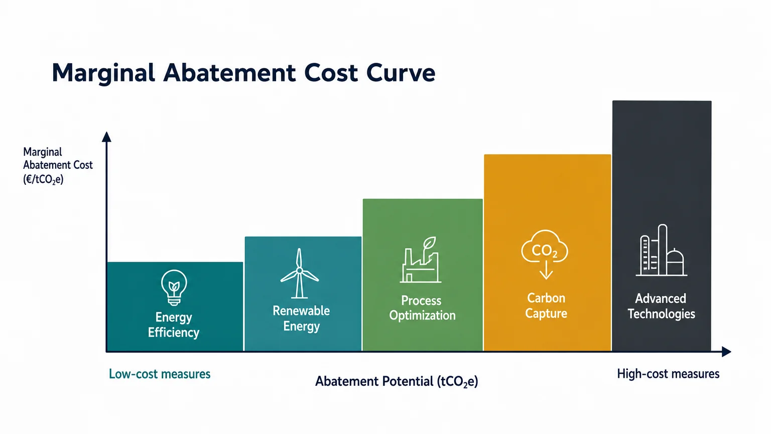
A marginal cost of abatement curve helps you answer a practical question: which emissions reduction actions deliver the next tonne of avoided emissions at the lowest incremental cost? To explore the financial logic behind these decisions, you can also consult our marginal abatement costs guide.

The curve turns a complex portfolio of climate measures into a visual ranking. It can reveal cost-saving opportunities, identify expensive hard-to-abate measures, and show how a carbon price may change investment decisions. However, the result depends heavily on assumptions about technology, energy prices, timing, policy, and interactions between sectors.

What does a marginal cost of abatement curve show?

At its core, a marginal cost of abatement curve compares the cost of reducing one additional unit of emissions with the volume of reductions available. The cost is commonly expressed in currency per tonne of carbon dioxide equivalent, or tCO2e. The abatement volume usually appears on the horizontal axis, while the marginal cost appears on the vertical axis.

Each bar or segment represents a potential action. Examples include improving industrial efficiency, switching from fossil fuels to renewable electricity, electrifying transport, installing heat pumps, reducing methane leakage, or deploying carbon capture. The width of each segment indicates the action’s potential emissions reduction. Its height indicates the incremental cost per tonne.

Options below the horizontal axis have a negative abatement cost. They may reduce emissions while producing net savings over the period assessed. An efficiency project, for example, could require upfront investment but lower energy expenditure enough to outweigh that investment. Options above the axis require additional spending after the relevant savings and revenues have been included.

The segments are normally ordered from the lowest cost on the left to the highest cost on the right. This creates a visual merit order. Reading from left to right shows what could be implemented first if the objective is to achieve a specific reduction target at the lowest apparent cost.

A curve is not a price list for technologies. It is a model of incremental costs under specific assumptions.

How do you read the curve in practice?

Imagine that your organization must reduce 100,000 tonnes of CO2e over a defined period. You begin by reviewing the measures on the left side of the curve. If the first measures have negative or low costs, they may offer an attractive starting point. You then continue across the curve until the combined width of the selected measures reaches the reduction target.

The height of the final selected segment represents the marginal cost of meeting that target within the model. It does not represent the average cost of the entire program. The average cost may be lower because earlier measures were cheaper. The total cost is better understood by considering the area under the curve across the selected abatement volume.

This distinction matters for investment decisions. A measure with a high marginal cost may still be necessary if lower-cost measures cannot deliver enough reductions. Conversely, a low-cost measure may have limited strategic value if it delays infrastructure changes that will be required later.

You should also check whether the curve uses annual or cumulative abatement. An annual curve shows the reduction available in a particular year. A cumulative approach considers reductions over a longer period. These two views can produce very different priorities because an action may have modest annual savings but substantial value over its operating life.

How is a marginal cost of abatement curve built?

Building a reliable curve begins with a baseline. The baseline describes what emissions, energy use, production, and costs might look like without the additional abatement action. Every opportunity is then compared with that reference case.

For each measure, analysts estimate several inputs:

• Capital expenditure and financing costs
• Operating, maintenance, and fuel costs
• Expected lifetime and utilization rate
• Energy prices and carbon prices
• Emissions avoided or removed
• Implementation constraints and technical potential
• Co-benefits, such as improved reliability or reduced air pollution

The basic calculation compares the additional cost of the measure with the emissions avoided. A simplified formula is:

Abatement cost = additional lifetime cost ÷ avoided emissions

In a more detailed model, the calculation may include discounting, changing energy prices, residual asset value, financing conditions, and interactions with other technologies. The selected assumptions determine whether a measure appears below or above the zero-cost line.

Analysts can create a curve using expert assessments of individual opportunities or through an integrated energy and economic model. The first approach is easier to explain and can be useful for project screening. The second approach can represent market feedback, technology substitution, and economy-wide effects more realistically, although it requires more data and more complex assumptions.

Why does the curve usually rise as abatement increases?

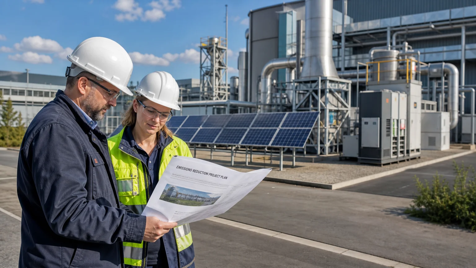
The first reductions are often easier to achieve because they rely on mature technologies, operational improvements, or projects with clear financial savings. As those opportunities are exhausted, deeper reductions may require new infrastructure, lower-carbon fuels, process redesign, or technologies that are not yet available at commercial scale.

This creates an upward-sloping curve in many analyses. The next tonne can become more expensive because it requires a more complex intervention than the previous tonne. Industrial facilities may need to replace equipment before the end of its useful life. Power systems may need additional transmission, storage, or firm low-carbon capacity. Heavy transport may require charging networks, alternative fuels, or redesigned logistics.

The curve can also change when external conditions change. Higher fossil fuel prices may improve the economics of electrification. Lower renewable energy costs may reduce the cost of switching power sources. A stronger carbon price can increase the cost of continuing to emit, making abatement investments more attractive even when their direct project cost remains unchanged.

Technology learning can shift the curve over time as well. A measure that appears expensive in one year may become more competitive after manufacturing capacity, supply chains, and workforce skills develop. This is one reason you should avoid treating a single curve as a permanent ranking of all climate technologies.

What are the main limitations of a MAC curve?

A curve can look precise even when its underlying estimates are uncertain. The model may use forecasts for fuel prices, technology costs, utilization rates, policy conditions, and emissions factors. Small changes in these inputs can alter the order of the measures and the apparent cost of reaching a target.

Another issue is that measures do not always operate independently. The emissions benefit of an electric vehicle depends partly on the electricity system. The value of a heat pump depends on building performance, electricity prices, and grid emissions. Industrial electrification may increase power demand and create new requirements for generation, transmission, and flexibility.

Timing also matters. A measure with a higher immediate cost may be important because it takes years to scale. Waiting can increase the future cost of deployment if supply chains, permitting systems, or skilled workers cannot expand quickly enough. A narrow curve focused only on today’s marginal cost may therefore undervalue early action.

The academic literature has described MAC curves as useful illustrations, but has also warned against relying on them alone. A peer-reviewed MAC curve study identified concerns involving uncertainty, interactions between sectors, ancillary benefits, and time-related effects.

Distributional effects can be missed as well. Two measures may have similar costs per tonne but very different consequences for households, workers, regions, or industrial competitiveness. A robust investment process should therefore combine cost analysis with feasibility, equity, resilience, and regulatory considerations.

How can carbon prices interact with the curve?

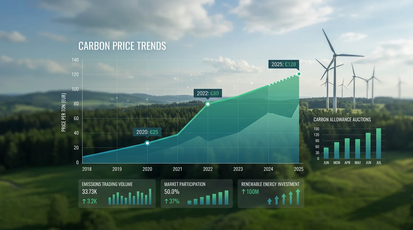
Carbon pricing changes the financial comparison between emitting and reducing emissions. When an organization faces a carbon cost for each tonne emitted, an abatement project becomes more attractive when its effective cost is below the expected cost of continuing to emit.

For example, suppose a measure has a marginal abatement cost of $70 per tCO2e. If the relevant carbon price and other avoided costs exceed that amount, the project may become financially rational. If the carbon price remains below the project cost, the organization may delay the investment unless regulation, incentives, operational needs, or strategic considerations provide another reason to proceed.

This does not mean that a carbon price automatically equals the correct abatement cost for every project. Allowance prices, taxes, internal carbon prices, and shadow prices serve different purposes. Their relevance depends on the jurisdiction, market design, compliance obligations, contract structure, and expectations about future policy.

For participants in emissions markets, the curve can provide a framework for interpreting supply and demand. It can help you consider how compliance entities may respond to allowance prices, technology investment, production changes, or hedging needs. Our explanation of how the emissions trading system supports the low-carbon transition provides additional context on this relationship.

What does recent research reveal about changing curves?

Recent research reinforces the importance of technology interactions. In a 2026 study of China’s coal power fleet, an interaction-aware model found that the cost-optimal technology mix changed as mitigation deepened. The study estimated approximately 1.2 gigatonnes of annual mitigation at negative marginal cost within its modeled system, while carbon neutrality required a marginal cost of US$56 per tCO2e under its assumptions. These results apply to that specific fleet and model, not to the global economy.

The example illustrates an important point. A curve is not only a ranking of isolated projects. It can also represent a sequence in which one investment changes the cost or potential of another. Energy conservation may be prioritized at an earlier stage, while biomass co-firing or carbon capture becomes more relevant at deeper levels of reduction.

Different models can produce substantially different estimates for the same target. An Australian government review of economic studies reported wide variation in modeled abatement costs, with differences linked to model structure, assumptions, and scenario design. You can review the Australian abatement review for an example of this modeling uncertainty.

For decision-makers, the practical response is not to reject the curve. It is to test several scenarios. You can vary energy prices, discount rates, carbon prices, technology costs, implementation speed, and the availability of supporting infrastructure. The most useful result is often a range of outcomes rather than one apparently exact number.

How should you use a marginal cost of abatement curve?

Start by defining the decision clearly. Are you trying to select projects for the next budget cycle, estimate the cost of a regulatory target, inform a carbon price, or build a long-term transition pathway? Each objective requires different boundaries, time horizons, and assumptions.

Next, separate screening from strategy. A curve is well suited to identifying attractive opportunities and comparing broad cost categories. It is less suited to deciding the full sequence of a multi-decade transformation without additional modeling.

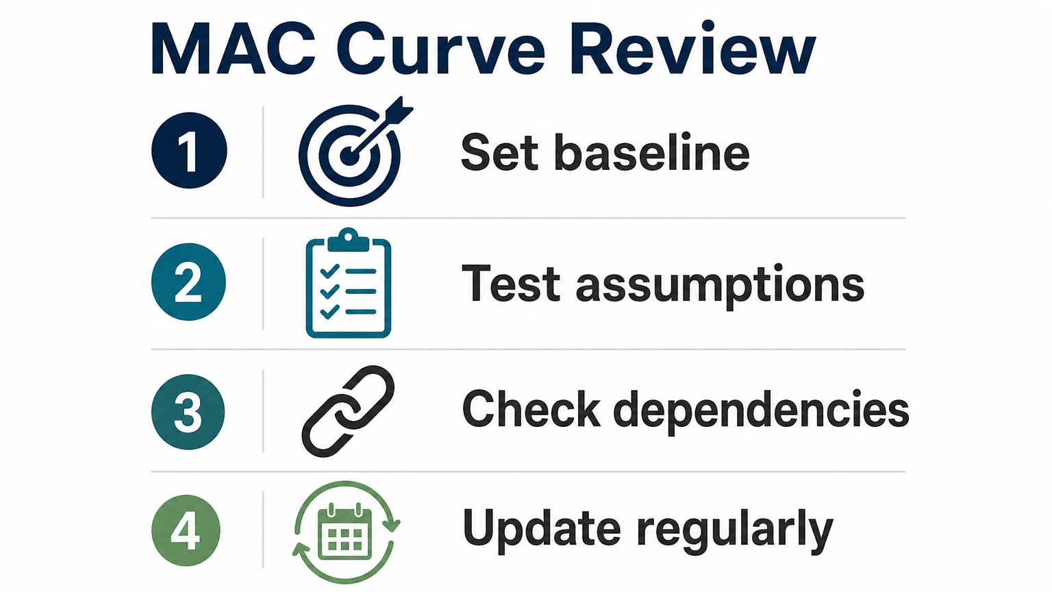
Use the following checks before acting on the result:

1. Verify the baseline: confirm that the reference scenario reflects realistic production, energy use, and policy conditions.
2. Test the assumptions: run sensitivity cases for prices, technology costs, financing, and emissions factors.
3. Check dependencies: identify whether one measure changes the cost, potential, or timing of another.
4. Include non-cost factors: assess permitting, supply chains, workforce availability, resilience, and social impacts.
5. Update the curve: revise it when market conditions, regulation, or technology performance changes.

For organizations active in carbon markets, data quality and execution also matter. A sound analytical view can lose value if prices are delayed, exposure is difficult to monitor, or risk limits are not applied before trading. We use tools such as real-time market monitoring, configurable alerts, API access, and pre-trade controls to help professional users connect market decisions with their operating processes.

Take action with Initiativ

Once you understand how abatement costs can influence allowance demand and compliance decisions, you need market infrastructure that supports timely analysis and controlled execution. The right tools can help you monitor prices, identify relevant market movements, and connect trading activity with your risk process.

Initiativ provides carbon trading solutions for traders and corporates through a programmable exchange for EU Allowances in spot and derivatives form, including futures and options. You can access real-time pricing, configurable alerts, API connectivity, pre-trade risk controls, and trading from 1 EUA, subject to membership and onboarding requirements.