Marginal Abatement: Costs, Curves, and Climate Decisions

How much should you spend to reduce one more tonne of emissions? That question sits at the heart of marginal abatement. To connect the concept with practical carbon-market decisions, you can begin with our marginal cost of abatement curve guide.

The answer is rarely a single universal number. It depends on the technology, operating conditions, energy prices, policy, timing, and reduction target. A measure can create savings at one site and impose a cost at another. You therefore need to interpret marginal costs as decision tools, not permanent rankings of climate solutions.

What does marginal abatement measure?

Marginal abatement describes the cost of achieving one additional unit of emissions reduction. In climate analysis, that unit is often one tonne of carbon dioxide equivalent, or tCO2e. The measure can be positive, zero, or negative.

A positive value means the next reduction requires a net expenditure. A negative value means the reduction generates enough operating savings or other revenue to exceed its costs. Energy-efficiency improvements can sometimes fall into this category, although the result depends on assumptions about capital costs, energy prices, utilization, and the period being assessed.

The word “marginal” is important. It does not describe the average cost of an entire decarbonization program. It describes the cost of the next increment. If a facility has already adopted its easiest measures, its next reduction may require more expensive equipment, process redesign, infrastructure, or fuel substitution.

For a single project, the basic calculation is:

Abatement cost = additional lifetime cost divided by avoided emissions

Additional lifetime cost may include capital expenditure, maintenance, fuel, electricity, financing, and implementation costs. You subtract relevant savings, incentives, or operating benefits before dividing by the emissions avoided. The result is commonly expressed in currency per tonne of CO2e.

At a broader level, analysts use marginal abatement to compare many actions. These may include building efficiency, methane controls, renewable electricity, industrial process changes, electrification, fuel switching, carbon capture, or changes in production. Each action has a potential reduction volume and a cost attached to it.

In January 2026, the United States Environmental Protection Agency published state-level technical and economic estimates for non-CO2 greenhouse-gas mitigation. The report uses disaggregated marginal abatement cost curves to show how mitigation potential and cost can vary across locations, sectors, and modeled conditions, as described in the 2026 EPA report.

How do you calculate a marginal abatement cost?

Imagine an industrial site comparing two projects. The first project requires $500,000 and avoids 10,000 tCO2e over its useful life. Its simplified abatement cost is $50 per tonne. The second project requires $1 million and avoids 40,000 tCO2e, giving it a cost of $25 per tonne.

The second project appears more attractive on a cost-per-tonne basis. However, that comparison is incomplete without considering timing, operational disruption, implementation risk, asset life, and interactions between the projects. A project that looks inexpensive may depend on infrastructure that is unavailable. Another may unlock savings or enable later reductions.

A robust calculation should define the following elements:

• Baseline emissions: the emissions expected without the intervention.
• Project emissions: the emissions produced after implementation.
• Investment costs: equipment, construction, engineering, and installation expenses.
• Operating costs: energy, maintenance, labor, materials, and compliance costs.
• Financial benefits: energy savings, avoided fuel purchases, incentives, or additional revenue.
• Reduction period: the years over which costs and avoided emissions are measured.
• Discount rate: the method used to compare costs and benefits that occur at different times.

You should also state whether the calculation is private or social. A company may include only costs that affect its own budget. A public analysis may include health benefits, energy-security effects, employment, or wider economic impacts. These different perspectives can produce different marginal costs for the same action.

Uncertainty is equally important. Future energy prices, carbon prices, production levels, equipment performance, and regulations can all change the result. A single point estimate may therefore create false precision. Scenario analysis is more useful when you need to make a long-lived investment decision.

For a practical explanation of the terminology and calculation logic, you can also consult our marginal abatement costs guide. The central principle remains simple: compare the incremental cost of the next reduction with the volume and quality of emissions avoided.

How do you read a marginal abatement cost curve?

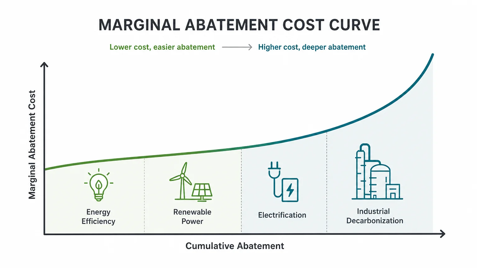
A marginal abatement cost curve normally combines two dimensions. The horizontal axis shows the quantity of emissions that can be reduced. The vertical axis shows the cost or saving associated with each reduction option.

Each bar, block, or segment represents a measure. Its width represents the measure’s potential emissions reduction. Its height represents the cost per tonne. Measures below the horizontal axis have negative costs, meaning they may create net financial savings. Measures above the axis require increasing levels of expenditure.

The options are generally arranged from the lowest cost on the left to the highest cost on the right. This creates a merit-order view. If you have a fixed budget, you can examine how far along the curve that budget may take you. If you have a fixed reduction target, you can identify the approximate cost of reaching it.

For example, a curve may begin with energy-efficiency projects that reduce emissions while lowering operating costs. It may then include renewable electricity, electrification, process changes, low-carbon fuels, and more expensive industrial technologies. The final segments may represent measures that are technically possible but commercially difficult.

The curve is useful for comparing choices, but it does not answer every strategic question. A bar can appear inexpensive because the analysis excludes grid constraints, permitting, supply-chain limits, workforce shortages, or the cost of coordinating several sectors.

You should also check whether the curve represents annualized costs, total costs, private costs, social costs, or a specific policy scenario. The same technology can appear in a different position when the analysis changes its assumptions. For a visual explanation of the structure, see our abatement curve guide.

Why is the cheapest measure not always the best path?

Suppose a company must reduce emissions by 10 percent within two years. The cheapest measures may be appropriate. Suppose the same company must reach near-zero emissions by 2050. The ranking may no longer provide a sufficient strategy.

This is the main limitation of a purely marginal approach. It favors the next least expensive reduction, while a deep transition may require early investment in technologies that are initially costly. Delaying those investments can create bottlenecks later, especially when equipment, grid capacity, industrial skills, or permitting take years to develop.

Actions also interact. A heat pump reduces emissions differently depending on the carbon intensity of electricity. The value of electric vehicles depends partly on charging infrastructure and power-sector changes. Industrial electrification may require transmission upgrades. These relationships mean that the cost and impact of one measure can change when another measure is introduced.

Timing matters as well. A measure that appears expensive today may lower future costs through learning, scale, supply-chain development, or infrastructure reuse. Conversely, a low-cost measure may become less valuable if it locks an organization into an asset that will need replacement before the end of its economic life.

The practical lesson is not to abandon marginal analysis. Instead, use it alongside a long-term transition pathway. Marginal costs help prioritize near-term actions. Scenario planning helps determine which capabilities, networks, and technologies must be developed before they become urgent.

You should ask four questions before accepting a curve’s ranking:

1. Does the measure support or obstruct the long-term emissions target?
2. Does its cost depend on another sector changing first?
3. Could implementation delays make the future pathway more expensive?
4. Does the analysis include operational, regulatory, and infrastructure constraints?

What can 2026 evidence tell you about changing costs?

Marginal abatement costs are not static. They change when technologies improve, energy prices move, regulations evolve, and markets create new incentives. They also change when better measurement reveals more reduction opportunities.

The International Energy Agency published a 2025 marginal abatement cost curve for methane from coal and updated the chart in April 2026. The IEA methane analysis illustrates how cost curves can be built for a specific gas, fuel source, and year rather than treated as universal climate rankings.

This specificity is valuable. Methane projects are assessed differently from carbon dioxide projects because the sources, monitoring methods, abatement equipment, leakage patterns, and time horizons differ. A curve for coal-mining methane should not be applied directly to industrial carbon dioxide reductions.

It is also useful to distinguish technical potential from economic potential. Technical potential describes what could be reduced with available measures. Economic potential describes what may be reduced under a selected cost threshold, policy framework, or market price.

When you review a 2026 study or dataset, check the reference year, geographic scope, emissions covered, baseline scenario, currency, discount rate, and treatment of co-benefits. A report published in 2026 may still model emissions and costs for 2025, 2030, or later years. The publication date and the modeled year are not interchangeable.

How does marginal abatement connect with carbon markets?

Carbon markets translate emissions constraints into financial signals. A company can compare the cost of reducing one more tonne with the cost of purchasing an allowance or credit. If internal abatement is cheaper, reducing emissions may be financially attractive. If the allowance is cheaper, procurement may be preferred, subject to compliance rules and long-term strategy.

This comparison is not a simple “reduce or buy” decision. Companies may need to manage compliance exposure, production changes, allowance inventories, price volatility, liquidity, and future regulatory requirements. The relevant question is often whether a reduction remains attractive across several price and operational scenarios.

A 2026 peer-reviewed study on firm-level and sectoral marginal abatement costs examines how these costs can relate to permit prices or required emissions taxes. The paper, available through a 2026 sector study, also emphasizes that marginal costs can vary across firms and sectors.

For professional participants, this creates a need for reliable market information and disciplined execution. A trader or procurement team may use marginal abatement analysis to estimate a preferred carbon-price range. The team can then compare that range with live allowance prices, available liquidity, forward exposure, and internal reduction plans.

Market access does not replace engineering analysis. A company still needs to validate the actual emissions reduction, project feasibility, and compliance treatment. However, carbon-market infrastructure can help connect the financial decision with execution, monitoring, reporting, and settlement.

How can you use marginal abatement in practice?

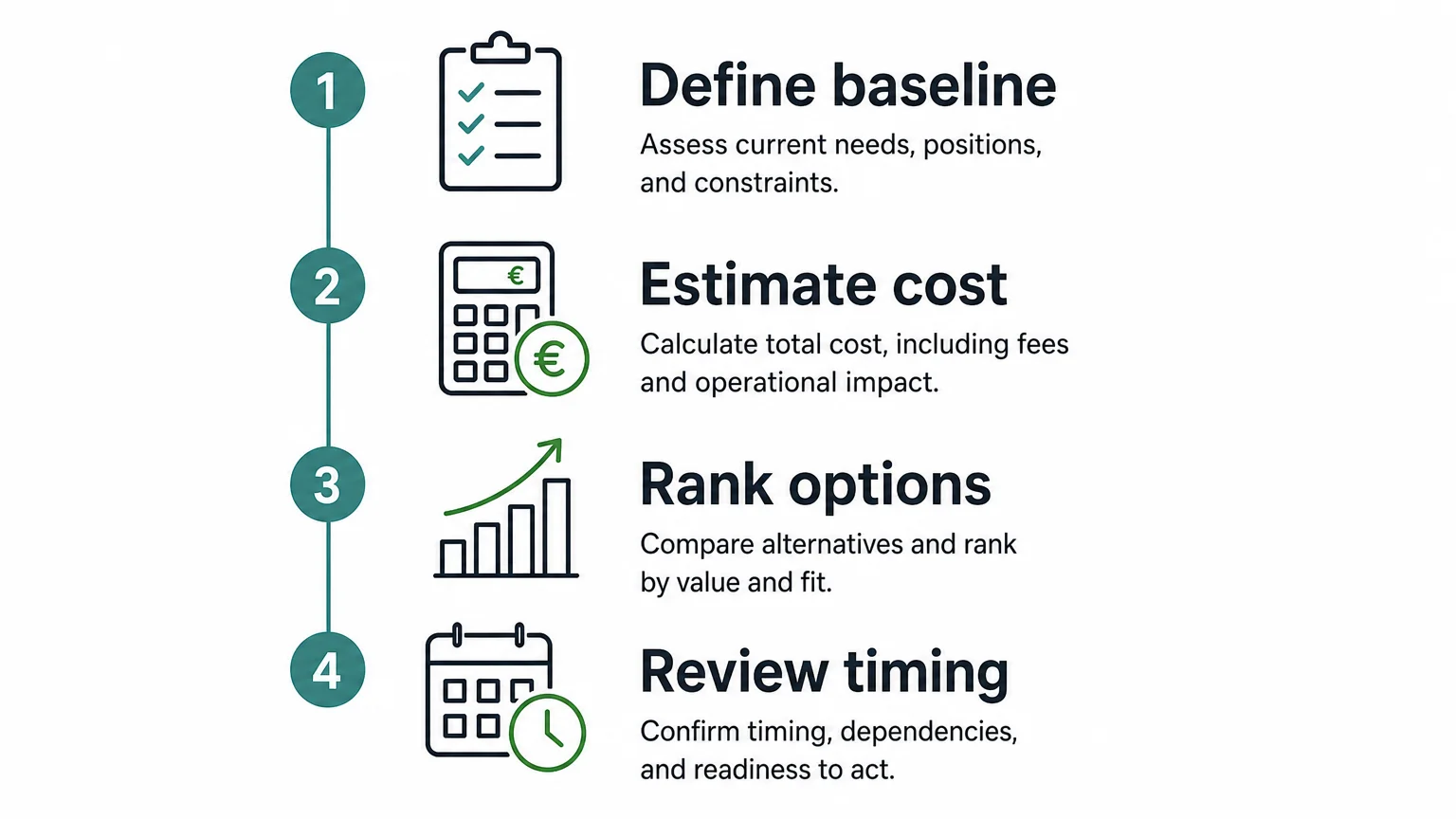
A practical workflow begins with a clear baseline. Define the activity, emissions boundary, reporting period, and expected operating conditions. Without a credible baseline, the calculated reduction may be overstated or difficult to verify.

Next, estimate costs consistently. Include capital expenditure, operating expenditure, financing, maintenance, energy use, incentives, and residual value. State whether you are using private or social costs, and identify the assumptions that could change the result.

Then, estimate the reduction potential. Do not compare a small project with a large project only by its cost per tonne. Consider the total tonnes avoided, implementation speed, permanence, monitoring quality, and compatibility with the organization’s wider transition plan.

After that, rank the options, but do not treat the ranking as final. Review interactions between measures, capacity constraints, procurement lead times, policy changes, and the risk of stranded assets. A slightly more expensive project may be preferable if it enables several later reductions.

Finally, connect the analysis to decision triggers. These may include an allowance price, a fuel-price threshold, a capital-budget limit, a compliance deadline, or a new technology milestone. Define what action follows when the trigger is reached.

For teams that also trade or procure EU Allowances, our abatement cost guide can help connect the terminology with practical cost analysis. You can then compare internal reduction opportunities with market exposure in a more structured way.

What are the main limitations to remember?

First, marginal costs depend on assumptions. Small changes in energy prices, utilization, discount rates, or technology performance can materially change the ranking. You should therefore treat the curve as a model output, not an objective law.

Second, the approach can overlook non-financial barriers. A project may have a low calculated cost but face permitting delays, limited suppliers, a shortage of skilled workers, or resistance from operational teams.

Third, curves can hide distributional effects. A measure that is inexpensive for one organization may impose costs on households, suppliers, workers, or communities. A cost-efficient pathway is not automatically fair or politically feasible.

Fourth, abatement quality matters. Avoided emissions estimates can vary in certainty, monitoring requirements, durability, and treatment under a specific emissions-trading system. You should verify the applicable rules before using an estimate for compliance or investment decisions.

Finally, a low marginal cost does not guarantee a low total transition cost. Large-scale decarbonization requires coordination across power, transport, buildings, industry, land use, finance, and public policy. Marginal analysis is most useful when it informs that broader strategy rather than replacing it.

Take action with Initiativ

Once you understand the cost of internal reductions, you may also need a reliable way to manage EU Allowance procurement, market exposure, and trading decisions. We help professional market participants connect analysis with structured access to carbon-market execution.

Our platform supports EUA spot and derivatives trading, live prices, order-book access, risk controls, API connectivity, position monitoring, reporting, confirmation, and settlement workflows. To evaluate how these capabilities fit your procurement or trading process, explore our carbon trading solutions for corporates.