Cost Abatement Curve: A Practical Guide for Carbon Markets

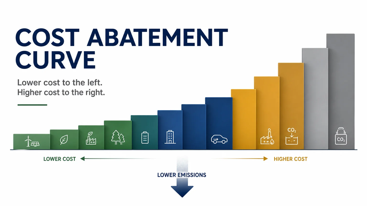
A cost abatement curve gives decision-makers a visual way to compare emissions reduction options by cost and potential. To connect that analysis with practical carbon-market decisions, you can also consult our marginal cost of abatement curve guide, which explains the relationship between abatement measures, costs, and carbon prices.

The basic idea is simple, but the interpretation requires care. A measure may appear inexpensive when considered alone, yet become less attractive if it depends on grid improvements, skilled labor, financing, or another technology. A reliable curve therefore supports decisions, but it should not be treated as a complete decarbonization strategy.

What does a cost abatement curve show?

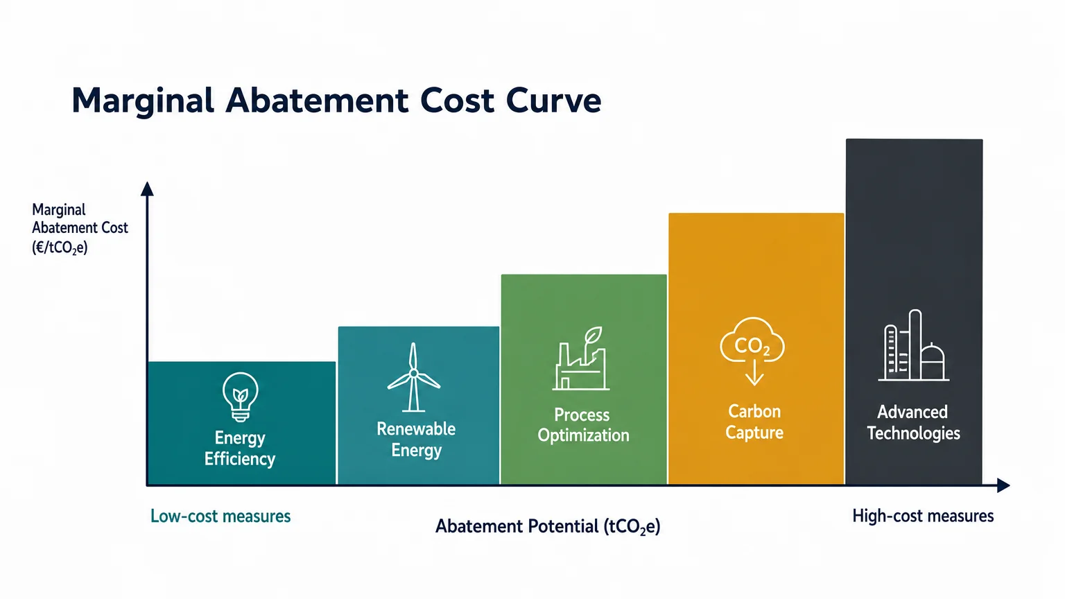
A cost abatement curve compares the cost of reducing one additional tonne of greenhouse gas emissions with the quantity of emissions that each measure could avoid. The cost is usually expressed in dollars or euros per tonne of carbon dioxide equivalent, written as $/tCO2e or €/tCO2e.

Each measure is commonly displayed as a bar or block. Its height represents the marginal abatement cost, while its width represents the estimated emissions reduction potential. Measures are usually ordered from the lowest cost on the left to the highest cost on the right. The resulting shape resembles a curve, although the underlying chart is often a sequence of rectangles.

Some measures can appear below the horizontal axis. These have a negative abatement cost, which means that their financial savings may exceed their implementation costs over the selected period. Energy efficiency improvements can sometimes fall into this category, especially when lower energy consumption creates continuing operating savings.

A negative value does not necessarily mean that the measure will be adopted immediately. Organizations may face capital constraints, limited information, operational disruption, procurement barriers, or competing investment priorities. The curve shows the modeled economics, not every condition that influences implementation.

How do you read the curve correctly?

Begin with the axes rather than the visual height of the bars. The horizontal axis normally shows cumulative emissions reduction, while the vertical axis shows the cost of reducing an additional tonne. Confirm whether the chart uses annual reductions, lifetime reductions, or a specific target year.

Next, identify the baseline scenario. A measure can appear more or less attractive depending on the technology, fuel mix, energy price, production volume, and operating assumptions used as the reference point. A heat pump, for example, may have a different abatement cost in a coal-intensive electricity system than in a low-carbon electricity system.

Then check the treatment of financing and operating costs. A robust curve should explain whether it includes capital expenditure, maintenance, fuel savings, financing costs, subsidies, taxes, carbon prices, and residual asset value. Two curves can rank the same technologies differently because they use different assumptions.

The width of a bar also deserves attention. A low-cost measure with limited technical potential may contribute less to a target than a higher-cost measure that can be deployed at scale. You should therefore examine both cost and cumulative reduction instead of selecting options based only on the lowest bar.

The IEA methane curve, updated in 2026 using 2025 data, illustrates how this method can be applied to a specific emissions source. Its presentation also shows why the unit of measurement, gas covered, geography, and time period must be clear before you compare results.

Why does it matter for carbon markets?

Carbon markets create a financial signal for emissions. When the market price of an allowance is higher than the modeled cost of a reduction measure, reducing emissions may be more economical than purchasing additional allowances. When the allowance price is lower, continuing to buy allowances may appear financially preferable, subject to regulation, operational constraints, and future price expectations.

This relationship is not automatic. An allowance price is a market observation, while an abatement cost is a modeled estimate. The two values may differ because of uncertainty, transaction costs, installation delays, production requirements, or differences between a company’s assets and the assumptions used in the curve.

A 2026 Stanford study on European cement producers found that an allowance price of €85 per tonne, observed on average in 2023, encouraged reductions of about one-third relative to the modeled status quo. The study also found that the incentive increased sharply above €100 per tonne, as described in the Stanford research.

For an EU ETS participant, this analysis can support several decisions. You may compare the expected cost of operational changes with the cost of EUA procurement, evaluate exposure under different price scenarios, and estimate how a production change could affect your allowance position.

For a practical explanation of how these relationships are visualized, our marginal abatement curve guide provides additional context on cost ranking, emissions reduction potential, and carbon-market interpretation.

How do you build a company-level curve?

Building a useful curve begins with a defined objective. You might want to reduce direct emissions from one facility, evaluate an EU ETS compliance plan, compare projects across a business unit, or test how a carbon price could affect investment decisions. The objective determines the scope, time horizon, and level of detail required.

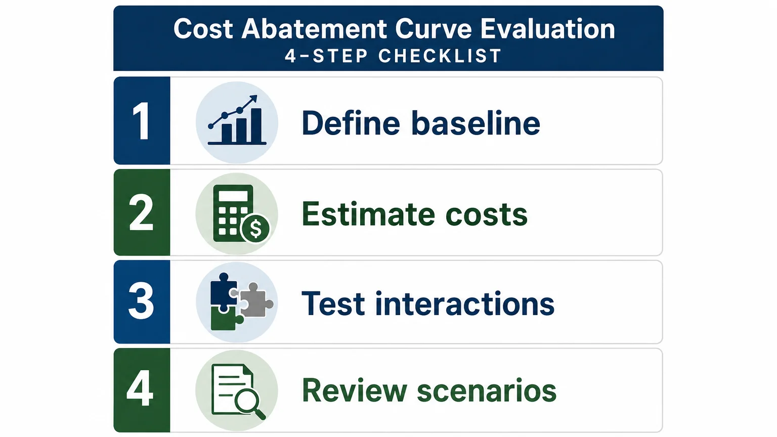
1. Define the baseline. Record current production, energy use, fuel mix, emissions, operating costs, and expected activity levels without the proposed measure.
2. List reduction measures. Include efficiency projects, fuel switching, electrification, renewable power, process changes, material substitution, carbon capture, and other relevant options.
3. Estimate each measure. Calculate capital costs, operating costs, savings, expected lifetime, implementation time, and potential annual emissions reduction.
4. Calculate the cost per tonne. Divide the discounted incremental cost by the expected emissions reduction, while documenting the discount rate and accounting period.
5. Rank the measures. Order the options from lowest to highest cost and show cumulative reduction potential.
6. Test sensitivities. Recalculate the curve under different energy prices, carbon prices, production levels, technology costs, and implementation dates.

You can use our abatement cost guide when reviewing the calculation itself. The key is to preserve a clear audit trail so that every cost, emissions factor, and operating assumption can be challenged or updated.

For EU ETS participants, the curve should also connect with allowance management. That may include expected free allocation, surrender obligations, procurement timing, hedging needs, production forecasts, and the difference between spot and derivative exposure.

When can a cost abatement curve mislead you?

A curve can mislead when it treats every measure as independent. In practice, technologies interact. The emissions benefit of electrification depends on electricity supply, while the value of additional renewable generation may depend on demand from electrified processes, storage, and grid capacity.

Timing can also change the result. A measure with a high current cost may be necessary early because it requires workforce development, permitting, infrastructure, or gradual equipment replacement. Waiting until the final years of a transition can create capacity constraints and higher deployment costs.

Geography matters as well. The EPA state-level report, updated in January 2026, presents mitigation potential and costs at a more detailed regional level. This demonstrates why national or global averages may not reflect the economics of a particular facility or state.

Technology learning creates another limitation. A measure that appears expensive today may become more affordable after investment, manufacturing scale, infrastructure development, or improved performance. Conversely, a low-cost measure may face supply constraints when many organizations attempt to adopt it simultaneously.

A 2026 study of forest-based mitigation in 215 countries found that additional mitigation becomes progressively more expensive as land and restoration constraints tighten. The findings, available in the Nature study, reinforce the importance of modeling physical limits rather than assuming unlimited deployment.

For these reasons, a curve should be treated as a decision input, not a fixed ranking. You should combine it with engineering feasibility, regulatory requirements, supply-chain conditions, workforce capacity, social impacts, and the strategic value of developing future technologies.

How should you use the curve in 2026?

In 2026, the most practical use of a cost abatement curve is scenario planning. Instead of asking which measure is cheapest in isolation, ask which sequence of measures can meet your emissions objective while preserving operational resilience and financial flexibility.

Start with a short-term scenario that reflects current prices and available technologies. Then add scenarios for higher carbon prices, tighter emissions limits, changing energy costs, delayed projects, and faster technology deployment. This approach shows where your exposure is most sensitive.

For a trading or procurement team, the analysis should connect with live market information. A curve can indicate when abatement may become financially attractive, while market data can help you assess the cost and timing of purchasing allowances. The two tools answer different questions and work best together.

Our platform supports professional participants that need to connect carbon-market decisions with execution and oversight. Through our abatement curve guide, you can review the analytical foundation, then apply the conclusions to procurement, risk, and position-management workflows.

A disciplined review process should include four checks. Confirm that the baseline is current, verify the emissions factors, challenge the deployment assumptions, and compare the result with operational plans. You should also record which decisions are reversible and which require long-lived infrastructure.

Take action with Initiativ

Once your abatement analysis identifies likely procurement needs, you need a reliable way to monitor exposure and execute carbon-market transactions. Professional participants can connect their planning process with market access, risk controls, and post-trade workflows.

Initiativ provides carbon trading solutions for traders and corporates, including EUA spot and derivatives access, live price monitoring, configurable alerts, API connectivity, position management, and reporting. The platform also supports confirmation and settlement workflows for eligible professional participants.